Linear Regression
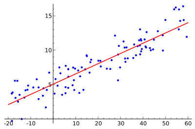 Linear regression is the "Hello, World!" of machine learning. It is one of the most basic ML algorithms and generally the first one taught. It is a simple parametric model with one learned parameter per input dimension plus a single bias parameter for the entire expression. As the name would suggest, it is a regression problem, so we will expect the output values to be continuous floats. It is also a linear algorithm, meaning that the relationship between the inputs and the output will always be linear. The function learned won't be able to produce curves or lines, and in turn, won't be able to accurately represent curved, non-linear data in the wild. But its a great place to start and you'd be surprised how many problems have data distributions that really are close to linear.
Uses
Linear regression produces a scalar output y from a vector of n-dimensional inputs, X (n, being a positive integer). There are two basic uses for linear regression:
- If the goal is prediction, linear regression can be used to fit a predictive model to an observed data set of
X and y values. After developing such a model, if an additional value of X is then given without its accompanying y value, the fitted (trained) model can be used to make a prediction of the value of y. This is perhaps the most common use case for supervised machine learning in general.
- Given a variable
y and a number of variables X1, ..., Xp that may be related to y, linear regression analysis can be applied to quantify the strength of the relationship between y and the Xj, to assess which Xj may have no relationship with y at all, and to identify which subsets of the Xj contain redundant information about y.
The Algorithm
Each output y is calculated by scaling each input X1, X2... by a coefficient (multiplier) M1, M2... and summing them with an additional single bias term b, therefore, y = MX + b. This function may look familiar, as it is very similar to the function that describes a line, only adapted to include multiple-dimensions, forming a hyperplane. y is predicted by a linear combination of the input values X. Great, now we've got a simple method of accurately predicting an output value as a combination of input values, provided their real-world relationship is linear. But how do we find the optimal parameter values for M and b?
Model Fitting
Enter model fitting, a fancy name for training. The idea is that you find, or "fit", model parameters that approximate a function to match your example training data. We use an optimization algorithm to find optimal values of M and b given enough example X and y values. We do this by minimizing an error function that describes the difference between our target values y and the predicted values y^ produced during the iterative training process, essentially quantifying how "wrong" the model predictions are from the real values. This error is computed using a loss function. The loss function often used with linear regression is Mean Squared Error (MSE). MSE computes the loss of a collection, or mini-batch, of examples as the average sum of the squared distances between the predicted values and the target values.
This is the function we hope to minimize using a standard optimization algorithm. When training begins, all model parameters are initialized to a random value. The goal of training is then to iteratively update each model parameter by a small amount in the direction that yields a lower value from the loss function. That is what we mean when we say "minimize" the loss function. The basic method we use to perform this optimization is called Stochastic Gradient Descent (SGD) and it is one of the foundational algorithms used in modern machine learning. It has many variants, but the idea behind all of them is the same. The value of each model parameter is iteratively updated by a tiny value that moves it in the direction pointed to by the derivative of its change to the error with respect to the input. The vector of all parameter derivatives is called the gradient, and it describes a multidimensional loss surface. If that all sounds like too much to handle right now, don't worry about it. You don't have to know how this works in order to leverage the power of high-level ML libraries and APIs.
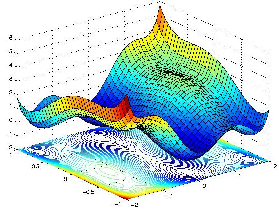 Gradient descent intuitively works like this: Imagine you are on a hike and you find yourself at the summit of the mountain just as the sun sets. You forgot to bring a flashlight and now you have to descend the mountain in the dark. You can't find the path and you don't remember the way down, so the best you can do is slowly take a step in the direction of steepest descent, ignoring global direction because you can't see. It might take a while, but provided the mountain has no high-altitude valleys, or local minima, you will eventually find your way back down to the bottom. Now substitute the topology of the loss function for that of the mountain and you've got an intuitive understanding of gradient descent. When the parameters are initialized the loss function lands at a random point in the N-dimensional parameter space. Iteratively updating the model parameters in the direction of nearest descent causes the values output by the loss function to be minimized and the overall accuracy of the model predictions to increase.
Example
Below is a small example of linear regression using scikit-learn. This example uses housing price data from ~500 homes in the Boston area during the late 1970s.
Each input sample has 13 features, and therefore is 13-dimensional. Below is a description of each feature:
- CRIM: per capita crime rate by town
- ZN: proportion of residential land zoned for lots over 25,000 sq.ft.
- INDUS: proportion of non-retail business acres per town
- CHAS: Charles River dummy variable (= 1 if tract bounds river; 0 otherwise)
- NOX: nitric oxides concentration (parts per 10 million)
- RM: average number of rooms per dwelling
- AGE: proportion of owner-occupied units built prior to 1940
- DIS: weighted distances to five Boston employment centres
- RAD: index of accessibility to radial highways
- TAX: full-value property-tax rate per $10,000
- PTRATIO: pupil-teacher ratio by town
- B: 1000(Bk - 0.63)^2 where Bk is the proportion of blacks by town
- LSTAT: % lower status of the population
- MEDV: Median value of owner-occupied homes in $1000's
Of our 506 samples, we want to hold out 20% to use as test data, leaving us with 404 samples with 13 features each (See Training vs Test data). We will use this 404x13 design matrix to fit our linear model (see Features and Design Matrices). Our target data y is the actual price of the home in thousands of dollars. We have 404x1 y values. You can find this example python script in code/python/linear-regression.py.
# "pip install scikit-learn" if you have not already done so
from sklearn import datasets
from sklearn.linear_model import LinearRegression
from sklearn.metrics import mean_absolute_error

# load boston housing data
data = datasets.load_boston()

# use %80 percent of the data for training and 20% for testing
y_train = data.target[0:int(len(data.target) * 0.80)]
y_test  = data.target[int(len(data.target) * 0.80):]
X_train = data.data[0:int(len(data.data) * 0.80)]
X_test  = data.data[int(len(data.data) * 0.80):]

model = LinearRegression(normalize=True)

print('[*] training model...')
model.fit(X_train, y_train)

print('[*] predicting from test set...')
y_hat = model.predict(X_test)

# print the results
for i in range(len(y_hat)):
    print ('[+] predicted: {:.1f}    real: {}     error: {:.1f}'\
           .format(y_hat[i], y_test[i], abs(y_hat[i] - y_test[i])))

print('[+] the mean absolute error is {:.1f}'.format(mean_absolute_error(y_hat, y_test)))
Linear regression models are very simple so the model should take no time to train and will begin to produce predictions like the ones below.
[*] training model...
[*] predicting from test set...
[+] predicted: 5.9    real: 8.5     error: 2.6
[+] predicted: 3.8    real: 5.0     error: 1.2
[+] predicted: 6.6    real: 11.9     error: 5.3
[+] predicted: 21.3    real: 27.9     error: 6.6
[+] predicted: 15.4    real: 17.2     error: 1.8
[+] predicted: 23.7    real: 27.5     error: 3.8
...
[+] the mean absolute error is 4.7
You can see that our model did alright, making an estimation that is $4,700 off from the real price on average. That said, we could likely improve greatly much over this baseline.
Next: Neural Networks and Deep Learning
Previous: Features & Design Matrices
Return to the main page.
All source code in this document is licensed under the GPL v3 or any later version.
All non-source code text is licensed under a CC-BY-SA 4.0 international license.
You are free to copy, remix, build upon, and distribute this work in any format for any purpose under those terms.
A copy of this website is available on GitHub.
