Model Architecture

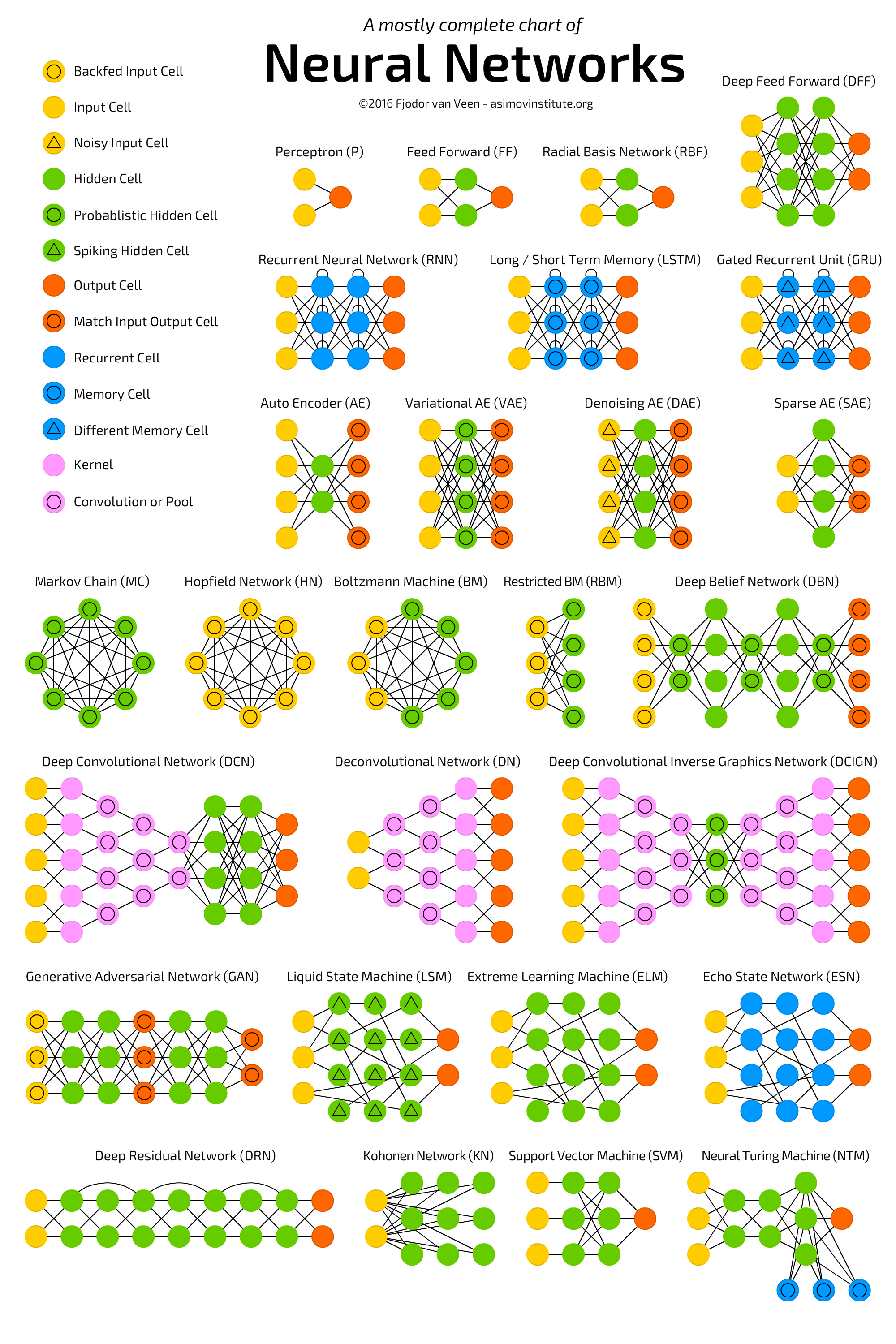
This tutorial series demonstrates how to build a machine learning pipeline from ideation to production. We'll use public tweets and transfer learning techniques to create a graphical application that generates Twitter bots. This chapter serves as an appendix, or forward, to the series; it broadly covers the topic of model architecture selection and design. In this chapter, we'll answer the question of which type of model should I use, and why?

Neural or Not

One of the first questions to ask when faced with any machine learning task is what class of algorithms to use to solve the problem? Will a linear model work or is the data being modeled non-linear? It's tempting to jump straight to the conclusion to use a neural network, but often a more basic model may work well, especially if you have access to very little training data. It's common practice to first choose a simple supervised learning technique, only moving to a more complicated model architecture like a neural net if the simpler method underperforms.

• Linear Regression + Logistic Regression: The most basic of linear modeling and supervised machine learning. Linear Regression is y = MX + b where y is predicted given a feature vector X, a set of learned weights M and a learned bias term b. Linear regression is used for regression tasks while Logistic Regression, despite its name, is used for classification tasks.
• K-Nearest Neighbors: This algorithm is wonderfully simple and can be used for both regression and classification. It is a model-less algorithm that predicts unseen values by measuring the euclidean distance between its input features and the input features of all of the training data.
• Decision Trees: These simple models are often used for classification. Decision trees can be thought of similarly to a flowchart or a hierarchy of "if, then" statements. Each leaf node in the tree represents a decision, or splitting path, while edges between the nodes represent the probabilities of each node being followed. Nodes at the bottom of the tree represent class membership. Decision trees are favorable because of their interpretability, however, they don't handle outliers very well, nor do they generalize well to large amounts of unseen data.
• Random Forests: Random Forest models are constructed using an ensemble of separate Decision Trees. For a classification task, the output mode of all Decision Trees is chosen as the output of the Random Forest model. For a regression task the output is an average over the output from all Decision Trees. Random Forests correct for the common problem Decision Trees have in of overfitting their training set.
• Naive Bayes classifier: Naive Bayes is a method of classification that utilizes the Bayes' theorem of probability with the naive assumption that input features are independent of one another. It has been used and studied extensively since the 1950s. It's performance has been found to be surprisingly good, even if the naive assumption of feature independence is incorrect, and very little training data exists. Naive Bayes is often used as a baseline model and is less complicated than SVMs.
• Support Vector Machines (SVM): These models excel at non-linear classification, although they can also be used for regression and linear modeling as well. These models were among the most popular techniques before the recent neural network resurgence and deep learning craze. SVMs use kernels to apply complex transformations to input features before learning decision boundaries using the transformed data. SVMs can be used as alternative methods to neural networks for non-linear modeling.

Each of these methods has found success in the field of machine learning and predictive modeling and I encourage you to experiment with these models. In the following tutorial, we'll favor a neural network approach to solving our problem, but these models are always a great place to start when approaching a machine learning solution or comparing your model's performance to that of other models.

Neural Network Architectures

The twenty-teens have seen a major resurgence in interest and success using neural networks and multi-layer perceptrons to solve complex machine learning problems. Some of this research has been categorized as under a new name: Deep Learning. Variants and adaptations of the vanilla neural network have been introduced, however all of these methods share common trates, and use the multi-layered perceptron at their core. All neural network models:

• Use activation functions at the output of one or more layer, causing the model to be non-linear.
• Involve one or more hidden layers defined in a hierarchy where the output of one layer is fed as the input to another layer.
• Have a number of input neurons equal to the size of each input feature vector.
• Have a number of output neurons equal to the number of predicted values or possible predicted classes.
• Optimize model weights via an external optimization algorithm dependent on a loss, or fitness, function.
• Use learned model weights to make predictions.
• Act as a black box, where data and state can be observed at the input and output layers, but becomes abstract and difficult to interpret at the hidden layers.
• Require lots of training data.

Beyond some of these common characteristics neural network architectures can differ. Below is a description of some of the most common neural network architectures.

Vanilla Neural Networks

Vanilla neural networks, or simply, neural networks are basic multi-layered perceptrons. They feature an input layer, one or more fully-connected hidden layers, and an output layer that is squashed by a sigmoid function if the output is categorical. For most neural network tasks, this will be the method of choice. Vanilla RNNs excel when dealing with:

• Non-sequential data
• Low(ish)-dimensional input (several thousand dimensions or less)

Convolutional Neural Networks

Convolutional neural networks (CNNs) differ from vanilla NNs in that they have one or more layers that share weights across inputs. This quality allows them to learn to recognize patterns invariant to their position and orientation in the input. CNNs are used primarily for solving tasks in the image domain, although they have also seen recent success dealing with time-series data.

CNNs slide kernels, small matrices of weight groups, multiple times across different areas of the input data to generate their output. This allows kernels to respond to input data more in some locations than in others and detect features and patterns in regions of input space. Kernels are often followed by operations that pool, or average, their output, therefor reducing the computational complexity of the task through downsampling at each new layer. Several convolutional + pooling layers are common before the final convolutional output is concatenated, or flattened, together and fed to one or more fully-connected layers before the final output layer. CNNs excel when dealing with:

• High-dimensional spatial data in one or more dimension
• Image data

Recurrent Neural Networks

Recurrent neural networks (RNNs) differ from vanilla NNs in that they maintain a set of internal weights that can persist state across multiple batches of inputs. Neurons maintain connections to their own previous state, which allows them to perform well when tasks require time dependence or sequential input data. If your input data is sequential in some way, like time series stock data, natural language text or speech data, or a series of actions performed by a user, RNNs will likely be the NN architecture of choice.

While vanilla RNNs can be used, it's much more common to use an RNN variant that utilizes special units, like long short-term memory units (LSTM) or gated recurrent units (GRU). LSTMs offer a complex memory unit that has the capacity to learn when to store information for multiple time steps and when to release it from memory. RNNs use LSTM units to improve long-term dependence and fight the vanishing gradient problem across time-series dimensions.

RNN architectures are flexible and their configuration can vary dependent on the task at hand. They can be designed to:

• Receive a sequence and predict the next element in the sequence
• Receive a sequence and predict an output sequence
• Receive a single input and output a sequence
• Receive a single input (dependent on prior input) and output a single input

RNNs excel when dealing with:

• Sequential or time-series data
• Useful when a network should retain state, or "remember" its prior inputs

Beyond

Vanilla NNs, CNNs, and RNNs are among the most popular neural network architectures in use today, but they are by no means the only ones in use. A few particularly exciting architectures that we won't cover here, but that are worth a look include:

• Generative Adversarial Networks (GANs)
• Autoencoder Networks & Sequence-to-Sequence Autoencoders

The Asimov Institute has a great post called The Neural Network Zoo which introduces and visually compares a large set of neural network architectures.

I find it useful to think of neural network architectures not as concrete, separate entities, but rather as proven building blocks that can be used, possibly in combination with one another, to achieve some goal. Consulting the machine learning literature, you will find that all of these architectures share common ancestry and are often the product of a combination of proven ML techniques. These architectures are great starting points for research and engineering, but there is no reason you can't deviate from the norm in designing an ML pipeline or solution. In the next section, we'll introduce the famous character-level recurrent neural network (char-rnn), as well as some modifications we've chosen to make to the basic architecture in the subsequent chapters of the tutorial.

Char-RNN

Char-RNN is a language generation model popularized by Andrej Karpathy in 2015 in his popular blog post The Unreasonable Effectiveness of Recurrent Neural Networks. The model is trained using a text file and learns to generate new text in the style of the author of the training text.

Basic Char-RNN

The Char-RNN model that Karpathy introduced was originally written in Lua Torch, but many people have since forked, remixed, and re-implemented the original model architecture. I'll first describe the original model, before describing the changes we've adopted. The Char-RNN model that Karpathy proposed uses a sequence of one-hot encoded inputs and produces a categorical distribution over a single output class, which is sampled from to predict the next letter in the sequence. Here's what the original Char-RNN architecture looks like in pseudo-code.

    
// assuming 
//      - the training data has 112 unique characters
//      - two LSTM layers with 512 units each
// 32 one-hot encoded characters as input
InputSequence(32 * 112)
InputLayer({ input: 32 * 112, output: 512 })
LSTMLayer({ input: 512, output: 512 })
LSTMLayer({ input: 512, output: 512 })
OutputLayer({ input: 512, output: 112 })
// sample from the probability distribution over all 112 character classes 
// to select the single output character
prediction = Sample({ input: 112, output: 1 })

// optionally, `Dropout({ probability: 0.2 })` could be added after each 
// LSTMLayer() to prevent overfitting.
    

Some notable characteristics of Karpathy's Char-RNN model that differ from the one we'll be building in this tutorial series include:

• One-hot input
• A sequence of inputs generates a single output
• Identical model architecture for training and inference
• The output probability distribution is sampled from directly

At Branger_Briz, we've had quite a bit of experience with this standard Char-RNN model architecture. But for this tutorial, we chose to use a variant of this architecture as an excuse to cover more material, explore new territory, and hopefully produce a better performing model.

Our Char-RNN Model

The model architecture that we've chosen to use for this tutorial series is inspired by YuXuan Tay's yxtay/char-rnn-text-generation model repository. We've hard-forked his project, removed the bits that are unnecessary for our tutorial, and added some new code as well. Our Char-RNN model variant differs from Karpathy's in several ways:

• We chose a subset of 96 printable characters as input classes, instead of using the thousands of unique character classes present in the dataset.
• We use a sequence of word embeddings instead of one-hot values as input to the model.
• The output from our model during training is a sequence (using a time-distributed dense layer).
• We modify the batch size and sequence length of our model between training and inference.
• The output probability distribution is first truncated and re-scaled before being sampled from.

    
// Assuming 
//      - the training data has 96 unique characters
//      - A word embedding vector dimension of 64
//      - two LSTM layers with 512 units each

// ARCHITECTURE DURING TRAINING
WordEmbeddingLookUpTable({ input: 32, output: 32 * 64})
InputLayer({ input: 32 * 64, output: 512 })
LSTMLayer({ input: 512, output: 512 })
LSTMLayer({ input: 512, output: 512 })
TimeDistributedOutputLayer({ input: 512, output: 96 * 32 })

// ARCHITECTURE DURING INFERENCE
WordEmbeddingLookUpTable({ input: 1, output: 1 * 64})
InputLayer({ input: 32 * 64, output: 512 })
LSTMLayer({ input: 512, output: 512 })
LSTMLayer({ input: 512, output: 512 })
TimeDistributedOutputLayer({ input: 512, output: 96 * 1 })
prediction = Sample({ input: 96 * 1, output: 1 })
    

Return to the main page.

All source code in this document is licensed under the GPL v3 or any later version. All non-source code text is licensed under a CC-BY-SA 4.0 international license. You are free to copy, remix, build upon, and distribute this work in any format for any purpose under those terms. A copy of this website is available on GitHub.